Boundary saving-based automatic differentiation

The code of this section locates at examples/check_features/ADvsBS. This exmaples shows a workflow of performing full waveform inversion based on pure automatic differentiation (PAD) and boundary saving-based automatic differentiation (BSAD). The BSAD method is used to reduce the GPU memory usage by reconstructing the wavefield with boundary saving strategy during loss backpropagation.

Generate model and geometry
```
python generate_model_geometry.py
```
The srcipt generate_model_geometry.py will generate a 2 layer ground truth model and a smoothed version of it. The corresponding source-receiver pairs will be generated as well. A figure named model_geometry.png illustrate the true and initial model.
Generate observed data

The configure file of forward modeling lies in configs/forward.yml
```
sh forward.sh
```
The script forward.sh will genereate the observed data shot_gather.npy for inversion.
Perform PAD FWI and BSAD FWI

Set boundary_saving: true can reduce GPU memory usage.

Perform full waveform inversion with pure automatic differeniation.
```
sh inversion_AD.sh
```
Perform full waveform inversion with boundary-saving automatic differeniation.
```
sh inversion_BS.sh
```
The configure files can be found in acoustic_fwi/configs/inversion_AD.yml and acoustic_fwi/configs/inversion_BS.yml.

Compare the results between the two methods.
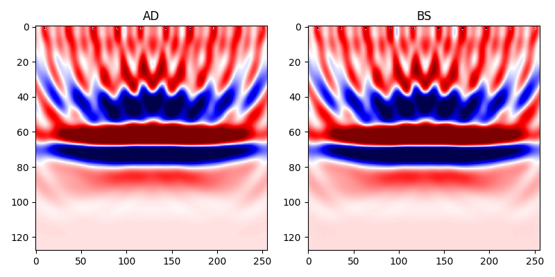
```
python AD_vs_BS.py
```
The BSAD method significantly reduces memory usage and sacrifices some computational efficiency. The gradients of the AD and BS methods are shown in the following figures.

2D Source Encoding Acoustic FWI

This chapter primarily focuses on how to perform Seistorch’s Source Encoding Full Waveform Inversion (FWI) using the same parameter file as Classic FWI. The difference lies in the utilization of codingfwi.py to perform the FWI process with source encoding. The files of this example are in folder examples/inversion/source_encoding/acoustic.

Generate the acquisition First you need to run the script the generate_model_geometry.py. Just like the other examples, it will generate sources.pkl and receivers.pkl which describes the acquisition of modeling.
```
python generate_model_geometry.py
```
Running forward modeling

Run the script forward.sh to generate the observed data.
```
sh forward.sh
```
Running inversion

The same configure file forward.yml is used for both forward modeling and inversion. The arguments of source encoding can be found in source_encoding_fwi.sh. The meaning of the arguments of codingfwi.py can be found in running commands.
```
sh source_encoding_fwi.sh
```
Show inverted results

The script show_results.py can be used to show the inverted results when the source_encoding_fwi.sh has been executed done.
```
python show_results.py
```

2D Source Encoding Elastic FWI

In elastic wave-equation based fwi, three model parameters are need for calculating lame parameters, i.e. vp, vs and rho. In this example, the rho is set to constant 2000. And the ratio between vp and vs is also a constant 1.73 except for the regions of sea with a depth of 500m. We only invert vp and vs in this example. The files of this example are in folder examples/inversion/source_encoding/elastic.

Files of true models all begin with true_, while initial models are prefixed with linear_. They are all placed in examples/models/marmousi_model.

Generate the acquisition

As with other examples, we need to first generate observed data. So we need a acquisition system. The script generate_mode_geometry.py can help you to do this.

We loaded the source at wavefield vz , which can be found in forward.yml. If you want to load the source to several wavefields, please refer to the section data format.

We record the velocity components vx and vz and use them for inversion.

The generated acquisition system is shown in the following figure.
Running forward modeling

Type the following commands in your conda environment, the observed data will be generated.
```
sh forward.sh
```
The generated data has a shape (nshots, nsamples, ntraces, ncomponents)(refer to data format). The following figure shows some randomly selected shots from vz.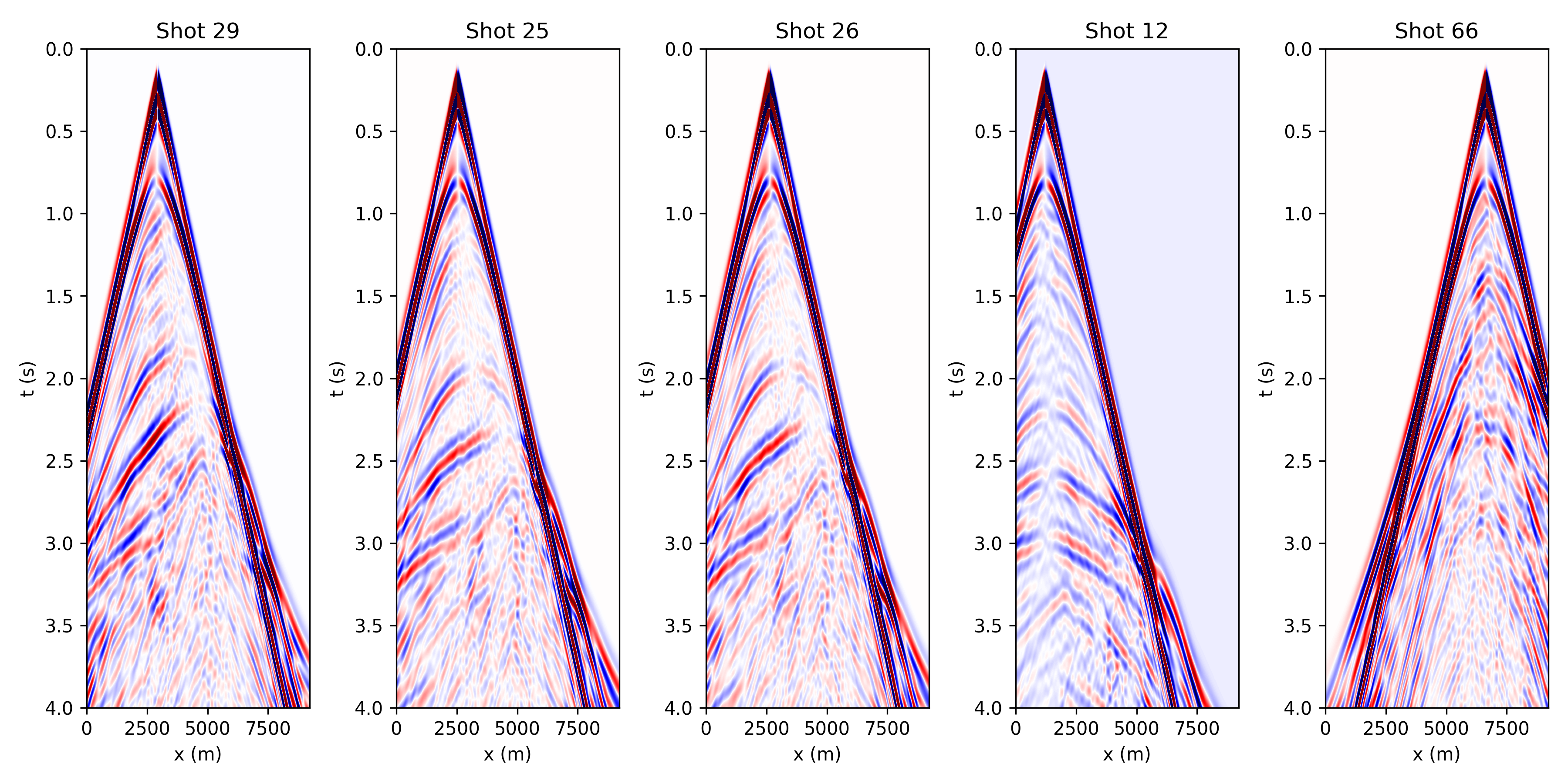
Running inversion

The same configure file forward.yml is used for both forward modeling and inversion. The arguments of this example can be found in source_encoding_fwi.sh. You can assign different loss functions (if they have been implemented in seistorch/loss.py) and learning rates to different parameters.
```
sh source_encoding_fwi.sh
```
Show inverted results

The script show_results.py can be used to show the inverted results when the source_encoding_fwi.sh has been executed done.
```
python show_results.py
```

Batched & Distributed FWI

WARNING: Please make sure there are more than 1 GPU on your machine for running this example successfully. (At least 2 GPU for this example)

In classic FWI codes, the computation of seismic data for each shot is typically done in a serial or MPI-parallel manner, meaning each shot is computed individually. However, deep learning frameworks provide us with batch computation capabilities through APIs like conv2d and conv3d. This allows us to simultaneously compute multiple shots, improving computational efficiency.

In Seistorch, both forward modeling and inversion provide batched computation (BC) functionality, but with different parameters. The BC is only valid for classic fwi, whose gradient are accumulated by multiples shots, while source-encoding-based fwi encoded several sources into a super-source so the gradient is calculated with only a super but single shot.

When running fwi.py for forward modeling you can specify the number of batches into which all the shots will be distributed by setting the num-batches parameter. This allows you to control how the shots are grouped for processing. More details can be seen in Running commands.

The source code of this section locates at examples/check_features/torchrun_dist. Please follow the following steps.

Generate geometry

The acquisition of this examples consists of 87 sources and 128 receivers in each shot.
```
python generate_model_geometry.py
```
Modeling observed data in a batched manner

In the forward.sh, we set --num-batches 10, it means that all shots will be separated into 10 bathches for modeling. Since we need to calculate 87 shots and use 2 GPUs (the host file is set as: 127.0.0.1:3), except for the last batch, which has a batch size of 7, the batch size for all other batches is 8.

Besides, all batches will be distributed to 2 GPUs equally. That is to say, GPU1 will run 1~5 batches and GPU2 will run the other 6~10 batches.
Perform classic fwi

For performing classic fwi, you need to set the minibatch in configure.yml to true, and set a proper batch_size which is 20 in our case. The number 20 represents the total shots used in one epoch for calculating the gradients. In this example, we use two GPU for fwi, so the nproc_per_node in inversion.sh need be set to 2.
```
batch_size: The number of shots used for gradient calculation in a single epoch.
The number of shots that each GPU need to perform = batch_size // nproc_per_node
The number of shots that each GPU need to perform at each step = batch_size // nproc_per_node // step_per_epoch
```
In the inversion.sh script, we specify step-per-epoch as 1, which bundles ten shots into a single batch for gradient computation on each GPU. This process is equivalent to separately computing the gradients for 10 shots and then summing them together.

If your model is too large, the number of shots in a single batch may be too large to fit into the GPU memory. There are two ways to solve this problem. One is to reduce the batch_size in configure.yml, and the other is to increase the step-per-epoch in inversion.sh. For the latter, the gradient will be accumulated for multiple batches, which will reduce the memory usage.
```
sh inversion.sh
```
Show the inverted results

The inverted resutls will be saved at ./results. The following figure shows the final inverted result.

Towed streamer data generation and inversion

In this chapter, we provide an example to illustrate the generation and inversion of towed streamer data. The source codes are in examples/inversion/towed/towed_2d.

In the seistorch, the sources and receivers are stored in a nested python list object (please refer to data format section). It’s flexiable for users to set a different number of receivers for different shots.

Note: It’s only necessary to ensure that the number of source points is the same as the number of receiver arrays; there’s no requirement for each receiver array to have the same quantity of receivers.

Model and acquisition setting

The script generate_model_geometry.py provides a workflow to generate a towed acquisition. We need to make sure that all the coordinates of sources and receivers are both within the model grids.

The generated acquisiton system looks like this:

In this example, we set the length of the cable to 2.56km with 128 receivers at an inverval of 20m. The interval between the source and the first receiver is 100m.

Type the following command in the example folder can generate the acquisition system:
```
python generate_model_geometry.py
```
Generate observed data
```
sh forward.sh
```
The generated data looks like this:

The placement of zero-offset traces on either the far left or far right depends on the arrangement of the horizontal coordinates in receivers.pkl.
Inversion

Run the script inversion.sh. A single node with 2 processors are used to perform full waveform inversion. A random mini-batch strategy with batchsize equals to 10 is used to accelerate the FWI. Ten shots are bundled together (set --num-batches 1) to further accelerate the inversion.

Note: The source-encoding fwi cannot be directly used for this type of data.
```
# Run inversion
sh inversion.sh
```
The inverted results will be saved at examples/towed_acquistion/results/towed. A python script named show_results.py can show the final inverted velocity model.
```
python show_results.py
```
The final inverted result is shown as follows:

Inversion with multiples

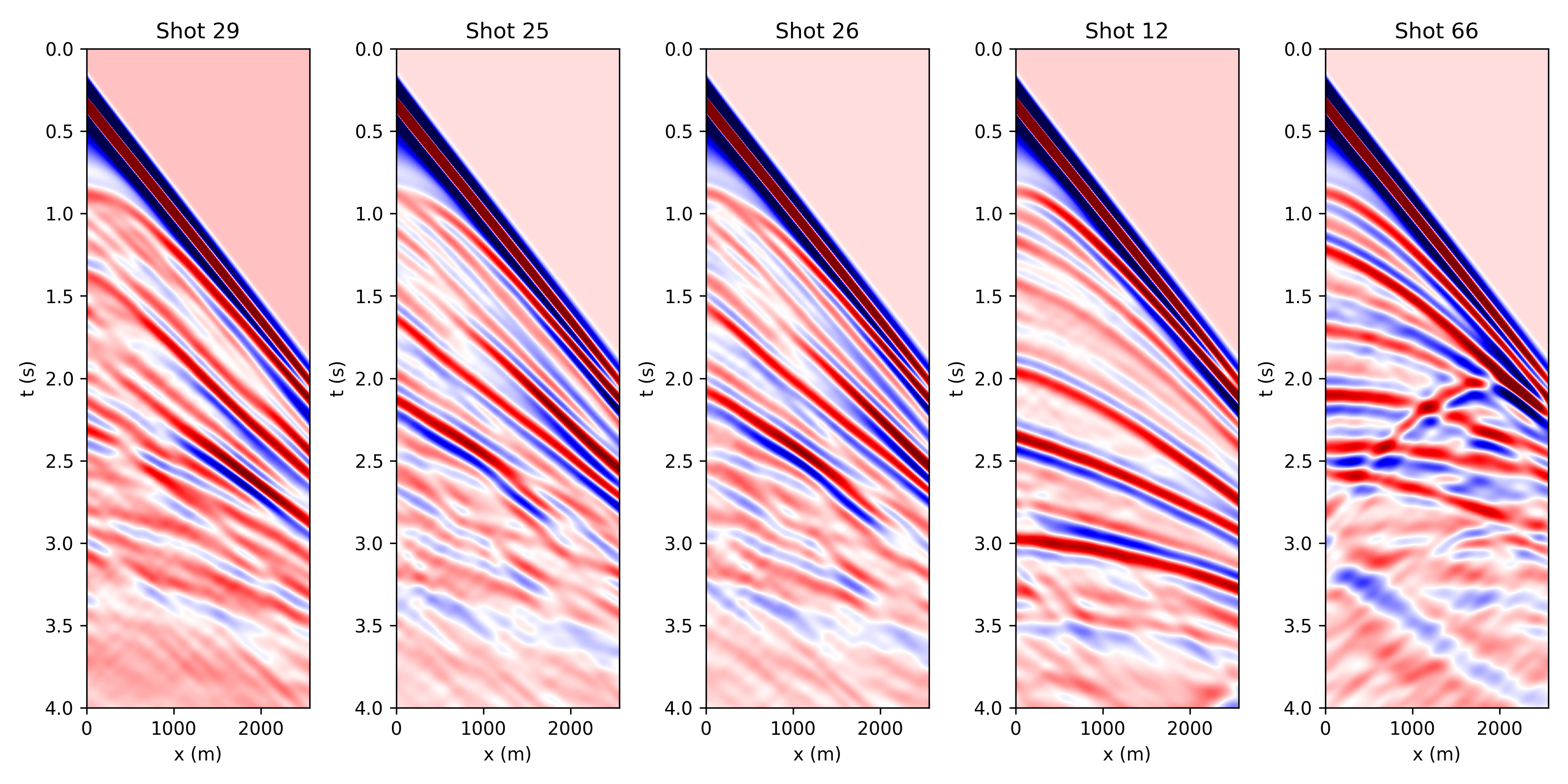
There is a bollean parameter named geom->multiple in configure file that can allow you modeling data with multiples. It simplely disables the top PML boundary for allowing waves propagating from boundaries.

This example shows a comparsion between the inversions with and without multiples. The configures of this example locates at examples/inversion/inversion_with_multiples.

Model and acquisition setting

The receivers are fixed at the bottom of the sea (the figure has been shown before in source encoding fwi). Typing the follow command in your terminal, it will genereate the geometry files for inversion.
```
python generate_model_geometry_fixed.py
```
Run forward modeling

You need to change directory to with_multiples and without_multiples and run the coresponding .sh file for generating the observed data with and without multiples.
```
cd with_multiples 
sh forward_withmultiple.sh
cd without_multiples 
sh forward_nomultiple.sh
```
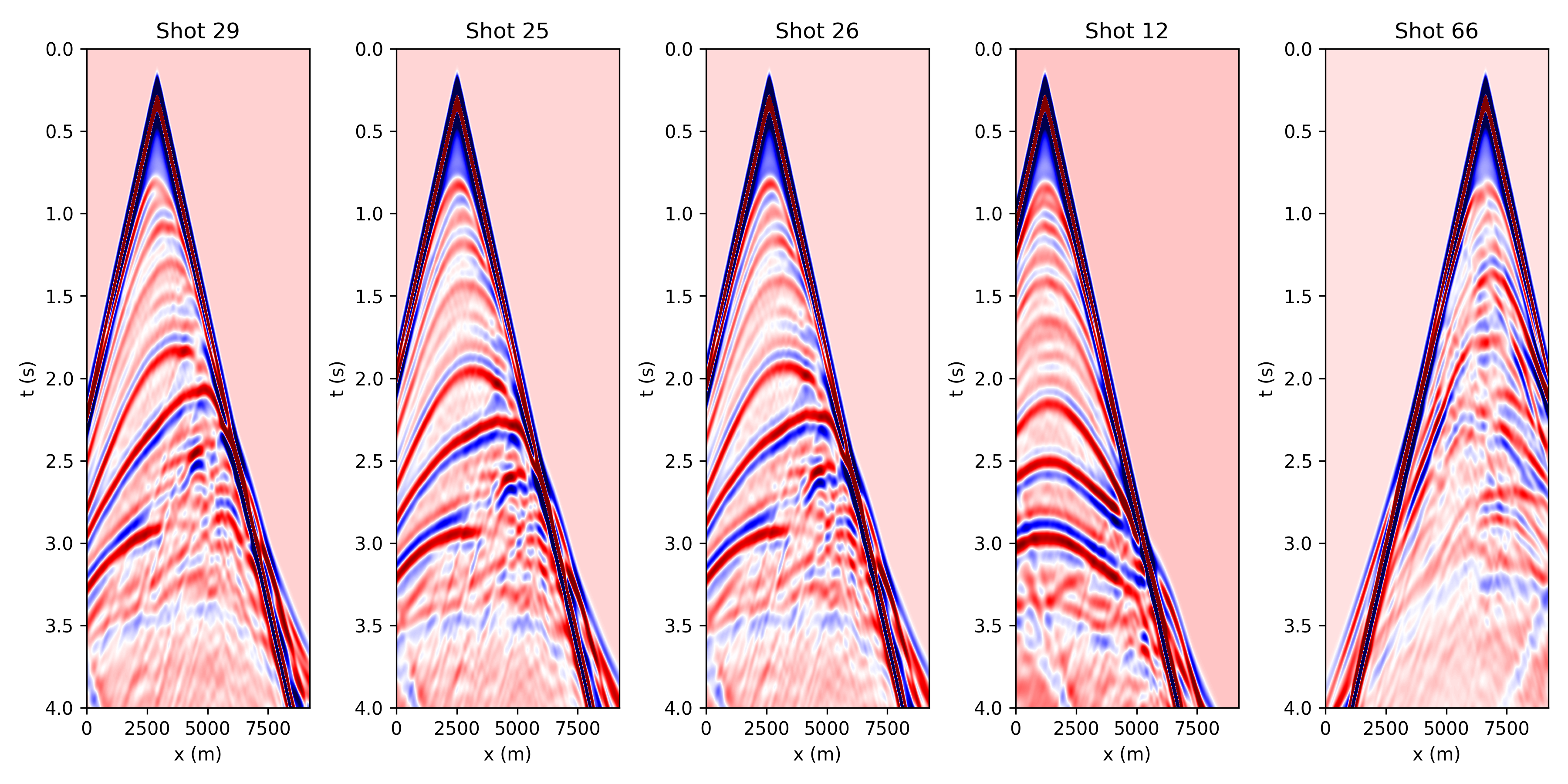
Then run the script show_shotgather.py, we will see the shot gathers with multiples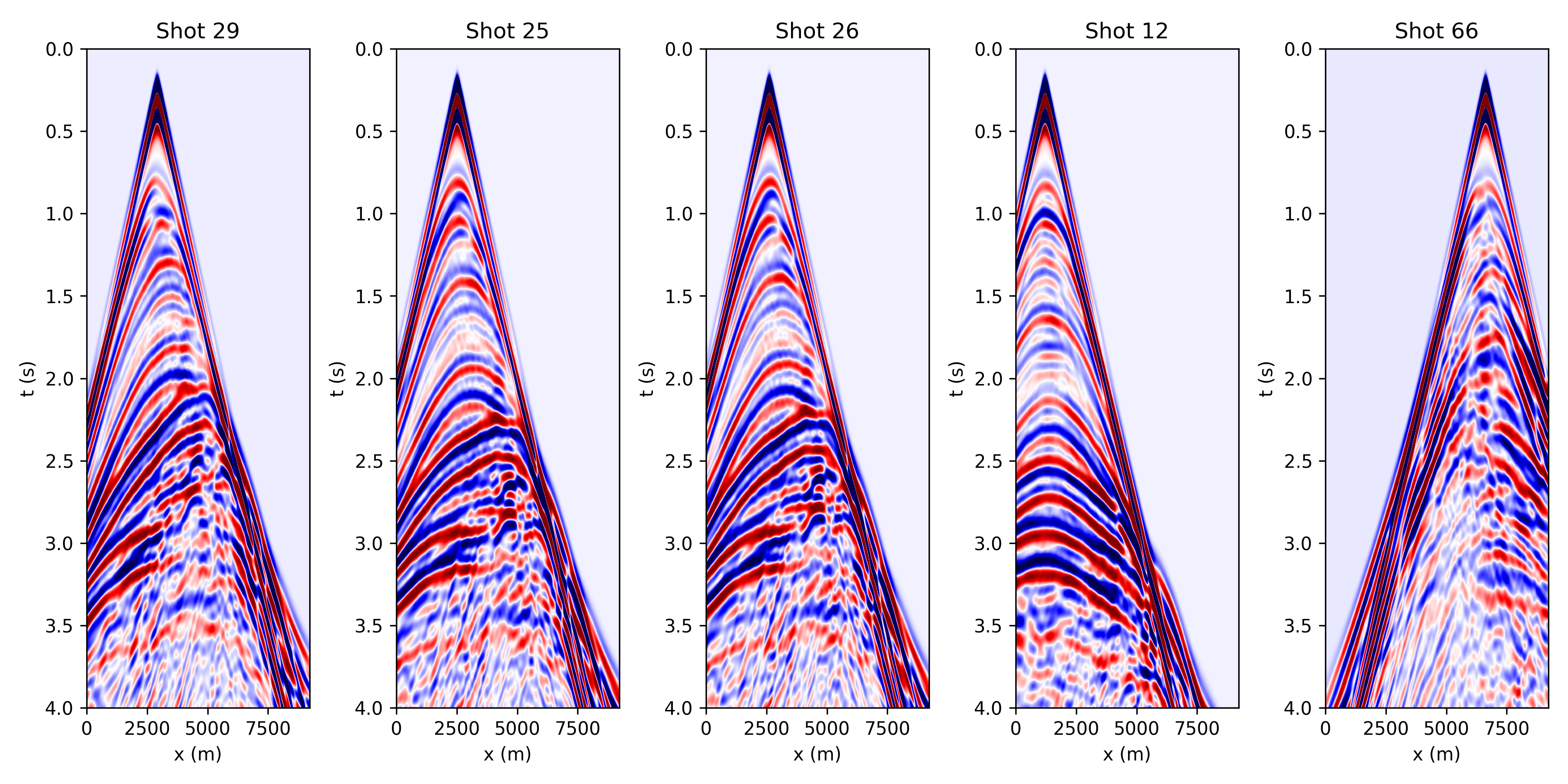

and shot gathers without multiples.
Run inversion

Run the inversion scipt in the two directories, respectively. The inversion results are shown as follows.