Advanced Customization

In Seistorch, advanced users have the flexibility to define and implement their custom wave equations and loss functions. This level of customization allows you to tailor Seistorch to specific research objectives and experiment with novel algorithms. This chapter will guide you through the process of creating your own wave equation and loss function.

Writing Your Custom Wave Equation

Step 1: Define the Wave Equation

• Objective: Clearly define the mathematical form of your custom wave equation, including the physical parameters, equations, and boundary conditions.

1. Define the needed parameters and names of wavefields: Added a new line in the class Parameters of seistorch/eqconfigure.py to configure your paramters.

   # seistorch/eqconfigure.py
   class Parameters:
       """ 
       Specify which model parameters are required by a given equation. 
       """
       @staticmethod
       def valid_model_paras():
   
           paras = {
               "my_wave_equation": ["c"]
           }
   
           return paras
   
   
   class Wavefield:
       """ 
       Specify which wavefield variables are required by a given equation. 
       """
       def __init__(self, equation="acoustic"):
           self.wavefields = getattr(self, equation)
   
       @property
       def my_wave_equation(self,):
           return ["wavefield1", "wavefield2"]
   
   

   The available source_type and receiver_type options will indeed correspond to the variable names defined within your Wavefield class.

   Example:

   geom:
   
       source_type: 
       - wavefield1
   
       receiver_type:
       - wavefield2
   

2. Define the Forward Timestep Function: Create a Python function named _time_step that adheres to the Seistorch solver interface and save it as my_wave_equation.py in seistorch/equations. You can set the parameter equation in configure file to my_wave_equation to call it.

   Example:

   # my_wave_equation.py
   def _time_step(*args):
       c = args[0] # vp
       wavefield1, wavefield2 = args[1:3] # wavefield variables
       dt, h, b = args[3:6] # dt: time sampling interval, h: grid size, b: boundary coefficients of PML
       # b = 0
       # When b=0, without boundary conditon.
       y = wave_equation_forward_in_time(wavefield1, wavefield2, c, dt, h, b)
       return y, wavefield1
   

   The _time_step function returns all the wavefield variables. In the scalar acoustic wave equation, the calculation typically involves using the wavefield values at time step t and time step t-1to compute the wavefield at time step t+1. The variables y and wavefield1 here represent the wavefield values at time step t+1 and time step t, respectively. These values are used to recursively compute the wavefield at each time step, and they are passed to the next iteration for the time-stepping.

3. Define the Backward Timestep Function: This step is optional. If you want to use boundary saving to save computational resources, please follow this step.

   Note: If you have sufficient computational resources, you can choose to only implement the _time_step function and set boundary_saving to false during inversion. This way, Pytorch will construct the computational graph automatically using the _time_step function in the forward modeling process.

   When performing fwi and the boundary_saving is set to true. Seistorch will save the necessary boundary values automatically during the forward modeling in the context of torch.no_grad().

   In the _time_step_backward, we will calculate the wavefields in reverse time. Assigning boundary values and reloading the source is essential for reconstructing the wavefield. The _time_step_backward is called in the context of torch.enable_grad().

   Example:

   # acoustic.py
   def _time_step_backward(*args):
   
       vp = args[0]
       wavefield1, wavefield2 = args[1:3]
       dt, h, b = args[3:6]
       boundary_values, _ = args[-2]
       src_type, src_func, src_values = args[-1]
   
       vp = vp.unsqueeze(0)
       b = b.unsqueeze(0)
   
       # b = 0
   
       # Calculate the wavefield at t-1
       y = wave_equation_reverse_in_time(wavefield1, wavefield2, c, dt, h, b)
   
       # Assign the boundary values
       y = restore_boundaries(y, boundary_values)
   
       # Add the source
       y = src_func(y, src_values, 1)
   
       return y, h1
   

Writing Your Custom Loss function

In Seistorch, adding a new objective function is typically easier than creating a wave equation solver. All objective functions should be implemented and placed in the seistorch/loss.py file. This way, you can easily access the new objective function by using a command like --loss vp=myloss” during the execution.

Example:

class MyLoss1(torch.nn.Module):
    def __init__(self, ):
        super(MyLoss1, self).__init__()

    @property
    def name(self,):
        return "myloss1"
    
    def forward(self, syn, obs):
        ctx.save_for_backward(syn, obs)
        return torch.nn.MSELoss()(syn, obs)

    def backward(self, grad_output):
        syn, obs = ctx.saved_tensors
        adj = 2*(syn-obs)*grad_output
        return adj, None

class MyLoss2(torch.nn.Module):
    def __init__(self, ):
        super(MyLoss2, self).__init__()

    @property
    def name(self,):
        return "myloss2"
    
    def forward(self, syn, obs):
        return torch.nn.MSELoss()(syn, obs)

In the functions mentioned above, you’ve defined two classes, MyLoss1 and MyLoss2, both of which inherit from torch.nn.Module. They each have a property attribute called name, and you can call the respective loss functions by accessing their name property.

However, it’s interesting to note that although you’ve defined a custom backward method in MyLoss1, when calculating gradients, the results are identical between the two loss functions. You can modify this code to implement your own custom backward method.

How to choose the value of num-batches?

The parameter num-batches determines how many shots are grouped together for calculation. If num-batches is set too low, it can decrease computational efficiency, while if it’s set too high, it may lead to out-of-memory (OOM) errors due to excessive GPU memory usage. We conducted several test runs for your reference.

We employed a layered model with a size of nz*nx=128*1024for forward modeling to test the computational efficiency under various conditions, including different batch sizes, node counts, and GPU numbers.

The following figure summarizes the efficiency. (CPU: Intel(R) Xeon(R) Silver 4214R CPU @ 2.40GHz; GPU: Tesla V100S-PCIE-32GB)

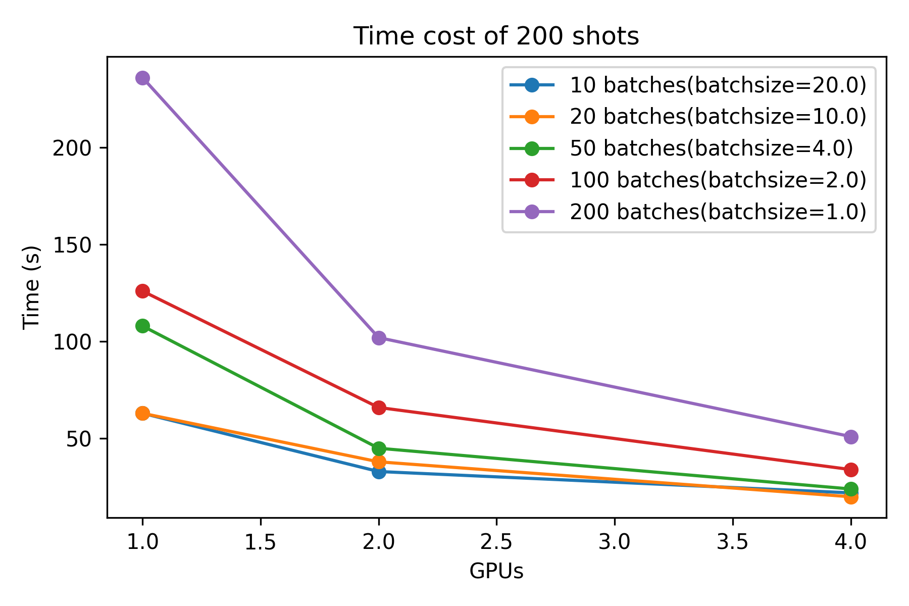
Note: When we had 4 GPUs, we utilized two nodes, each equipped with 2 GPU cards.